Here are some notes I took when reading the second edition of the Reinforcement Learning: An Introduction book.
If you want to get into Reinforcement Learning, or are just interested in Artificial Intelligence in general, I highly recommend that you read this book!
It does require some mathematical background to read and understand everything (mostly Linear Algebra, Probabilities, Statistics, and some Calculus), but it is overall one of the best - and most exhaustive - introductory books about Reinforcement Learning out there.

Chapter Index

1. Chapter 1: Introduction
2. Part I: Tabular Solution Methods
   1. Chapter 2: Multi-armed Bandits
   2. Chapter 3: Finite Markov Decision Processes
   3. Chapter 4: Dynamic Programming
   4. Chapter 5: Monte Carlo Methods
   5. Chapter 6: Temporal-Difference Learning
   6. Chapter 7: n-step Bootstrapping
   7. Chapter 8: Planning and Learning with Tabular Methods
3. Part II: Approximate Solution Methods
   1. Chapter 9: On-policy Prediction with Approximation
   2. Chapter 10: On-policy Control with Approximation
   3. Chapter 11: *Off-policy Methods with Approximation
   4. Chapter 12: Eligibility Traces
   5. Chapter 13: Policy Gradient Methods
4. Part III: Looking Deeper
   1. Chapter 14: Psychology
   2. Chapter 15: Neuroscience
   3. Chapter 16: Applications and Case Studies
   4. Chapter 17: Frontiers

Chapter 1: Introduction

Def. Reinforcement Learning (RL): an agent learns how to map situations to actions through trial-and-error or planned interaction with a (possibly) uncertain environment, so as to maximize a numerical reward value (i.e., achieve his goal or goals).

• Delayed reward is another important characteristic of RL, since any action taken may influence (not only the immediate reward value, but also) any subsequent rewards;
• RL can be formalized as the optimal control of incompletely-known Markov Decision Processes (MDPs).

Besides RL, other Machine Learning (ML) paradigms include Supervised Learning - predicting the correct label, given the corresponding set of features - and Unsupervised Learning - finding hidden patterns in a collection of unlabeled features.

A challenge unique to the RL paradigm is that of the trade-off between exploration versus exploitation. This challenge arises due to the fact that an agent prefers to take the actions that have previously given the highest rewards (exploitation), but it must also try out other actions in order to have more knowledge about which actions it should select (exploration).

A RL system has four main elements beyond the interactive agent and the environment, which are:

• A policy $\pi_t: s \rightarrow a$, which in stochastic cases specifies a probability for each action;
• A reward $r(s, a)$, an immediate signal that specifies how good it is for an agent to have chosen a certain action in a given state (may also be stochastic);
• A value function $v(s)$ that specifies the total reward an agent is expected to accumulate in the future if he starts at a given state, i.e., predicted long-term reward;
• A (optional) world model used by model-based methods (opposed to purely trial-and-error model-free methods) for planning.

Part I: Tabular Solution Methods

Chapter 2: Multi-armed Bandits

Non-associative setting: a problem setting that involves learning to act in only 1 situation.

Associative setting: a problem setting where the best action depends on the situation.

Section 2.1: A $k$-armed Bandit Problem

Setting of the $k$-armed bandit learning problem (analogous to a slot machine with $k$ levers):

1. Choose 1 action from among $k$ different options;
2. Receive a (numerical) reward from a stationary probability distribution which depends on the action selected;
3. Repeat steps 1 and 2 with the purpose of maximizing the expected total reward over some time period (e.g., 1000 action selections or time steps).

Value of an action: the expected or mean reward received if that action is selected

Letting $A_t$ be the action taken at time step $t$ and $R_t$ the corresponding reward, then the value $q^{*}(a)$ of an arbitrary action $a$ is given by:

Since we do not know the true value of each action, we need to estimate them in such a way that the estimates are close to the real values. The estimated value of an action $a$ at time step $t$ is denoted by $Q_t (a)$.

Greedy action: the action with the highest estimated value at a given time step

• Choosing this action equates to the agent exploiting his current knowledge of the values of the actions;
• Selecting 1 of the non-greedy actions enables the agent to improve his estimates of the non-greedy action's value, i.e., exploration;
• Exploitation maximizes the reward on 1 step, but it needs to be intercalated with exploration steps so as to maximize the greater total reward in the long term.

Section 2.2: Action-value Methods

Def. Action-value Methods: methods used to estimate the values of actions and to use those estimates to select an action to take at a given time step.

Letting $\mathbb{1}_{predicate}$ be the random variable which equals $1$ if the $predicate$ is true and $0$ otherwise, the value of an action can be estimated by averaging the rewards received:

If the denominator is zero (action has never been taken), then $Q_t(a)$ is defined as an arbitrary default value (e.g., zero). By the law of large numbers, as the denominator goes to infinity, $Q_t(a)$ converges to $q^{*}(a)$. This is called the sample-average method for estimating action values.

The simplest action selection rule is to always select a greedy action and - if there is more than 1 action with the same highest value - to break ties in some arbitrary way (e.g., randomly). This action selection method can be written as:

This selection method never performs exploration. A simple alternative that does so is to select the greedy action most of the time (probability $1 - \epsilon$) and (with probability $\epsilon$) to randomly select any possible action with equal probability. Methods that use this near-greedy action selection rule are dubbed $\epsilon$-greedy methods.

Section 2.3: The 10-armed Test-bed

Non-stationary setting: problem setting where the true values of the actions (or the reward probabilities) change over time.

Given a set of 2000 randomly generated $k$-armed bandit problems (with $k = 10$), for each problem in the set, the action values $q^{*}(a), \ a = \{1, 2, \dots, 10\},$ were selected from a normal (Gaussian) distribution with $\mu = 0, \ \sigma^2 = 1$. When a learning method is applied to this problem selects action $A_t$ at time step $t$, the actual reward ($R_t$) was drawn from a normal distribution with $\mu = q^{*}(A_t), \ \sigma^2 = 1$.

The performance of the learning methods is measured as it improves with experience over 1000 time steps of the bandit problem, which makes up a single run. To obtain an accurate measure of the learning algorithms' behavior, 2000 runs are performed and the results for the bandit problems are averaged.

A greedy action selection method is compared against 2 $\epsilon$-greedy methods (with $\epsilon = 0.01 \lor \epsilon = 0.1$). All methods begin with initial action-value estimates of zero and update these estimates using the sample-average technique.

While the greedy method improved slightly faster than the other 2, it converged to a reward-per-step of 1, which is lower than the best value of around 1.54 achieved by the $\epsilon$-greedy method (with $\epsilon = 0.1$). The method with $\epsilon = 0.1$ improved faster than the method with $\epsilon = 0.01$, since it explored more earlier. However, the method with $\epsilon = 0.01$ converges to a higher reward-per-step in the long run, since the method with $\epsilon = 0.1$ never selects the optimal action more than 91% of the time.
It is possible to perform $\epsilon$ annealing to try to get fast learning at the start combined with convergence to a higher reward average.

It takes more exploration to find the optimal actions in cases with noisy rewards (i.e., high reward variance), meaning that $\epsilon$-greedy methods perform even better in those cases, when compared to the greedy method. Also, although the greedy method is theoretically optimal in the deterministic case (i.e., with $\sigma^2 = 0$), this property does not hold in non-stationary bandit problems, making exploration a necessity even in deterministic settings.

Section 2.4: Incremental Implementation

For a single action, let $R_i$ denote the reward received after the $i^{th}$ selection of this action and $Q_n$ the estimate of its action value after it has been selected $n - 1$ times, written as:

Instead of maintaining a record of all the rewards and performing the computation for the estimated value whenever needed (resulting in the growth of both computational and memory requirements), we can devise incremental formulas to update the averages with a small and constant computation to process each new reward. Given $Q_n$ and the $n^{th}$ reward $R_n$, the new average of all $n$ rewards can be computed as:

This implementation only needs memory for $Q_n$ and $n$, and only performs a small computation for each new reward. The general form of the previous update rule is given by:

where $[Target - OldEstimate]$ is an error in the estimate, which is reduced by taking a step towards the (possibly noisy) target value. The step-size parameter is generally denoted by $\alpha$ or $\alpha_t (a)$.

def bandit_problem(k: int, epsilon: float, bandits):
    Q_a = [0]*k;
    N_a = [0]*k;
    while(True):
        if random_float(0, 1) <= epsilon:
            A = random_int(0, k)
        else:
            A = argmax(Q_a)
        R = bandits[A].get_reward()
        N_a[A] += 1;
        Q_a[A] += (1/N_a[A]) * (R - Q_a[A]);

Section 2.5: Tracking a Non-stationary Problem

When reward probabilities change over time, it makes sense to give more weight to recent rewards than to those receive long ago. This can be done by using a constant step-size parameter, e.g., for updating an average $Q_n$ of the $n - 1$ past rewards w.h.t.:

where the step-size parameter $\alpha \in \ ]0, 1]$ is constant. Given this, $Q_{n + 1}$ becomes a weighted average (since the sum of weights = 1) of the past rewards and initial estimate $Q_1$:

Since $1 - \alpha < 1$, the weight given to $R_i$ decreases as the number of intervening rewards increases. Also, the weight decays exponentially in proportion to the exponent on $1 - \alpha$ and, if $1 - \alpha = 0$, the entire weight goes onto the very last reward $R_n$. This method is sometimes called an exponential recency-weighted average.

Letting $\alpha_n (a)$ denote the step-size parameter to process the reward obtained after the $n^{th}$ selection of action $a$, for the sample-average method, w.h.t. $\alpha_n (a) = 1/n$, whose convergence to the true action values is guaranteed by the law of large numbers. However, convergence is NOT guaranteed for all choices of the $\{\alpha_n (a)\}$ sequence. Through a result in stochastic approximation theory, we obtain the conditions required to assure convergence with probability 1:

where the first condition is required to guarantee that the steps are big enough to overcome any initial conditions or random fluctuations that would otherwise result in getting stuck at saddle points, and the second condition guarantees that the steps will eventually become small enough to assure convergence.

The second condition is not met for the constant step-size parameter case, i.e., $\alpha_n (a) = \alpha$. This means that the estimates will never completely converge, which is actually a desirable property for non-stationary problems (the most common type of problem in RL), since the estimates continue to vary in response to the most recently received rewards, accounting for the changes in reward probabilities over time. Also, the sequences of step-size parameters that meet both of the above conditions often lead to slow convergence rates, meaning that these are seldomly used in applications and empirical research.

Section 2.6: Optimistic Initial Values

All previous methods are somewhat dependent on the initial action-value estimates $Q_1 (a)$, i.e., they are biased by their initial estimates. This bias decreases over time as various actions are selected. However, while for sample-average methods the bias eventually disappear after all actions have been taken at least once, the bias is permanent for methods with a constant $\alpha$.

This property means that, when using methods with a constant $\alpha$, the user must select the values for the initial estimates, which provides a way to supply some prior knowledge about the expected rewards, at the possible cost of being harder to tune.

By selecting optimistic initial action-values, i.e., $Q_1 (a) >> R_1 (a), \forall a$, the agent will always be disappointed since the rewards will always be far less than the first estimates, regardless of which actions are selected. This encourages exploration, as the agent will select all possible actions before the value estimates converge, even if greedy actions are selected at every single time step.

This technique for encouraging exploration is named optimistic initial values and is a simple, yet effective trick when used on stationary problems (e.g., with $Q_1(a) = 5$ it outperforms a $\epsilon$-greedy method with $Q_1(a) = 0$ and $\epsilon = 0.1$).

An important caveat is that, since the drive for exploration in the previous technique is dependent on the initials conditions and disappears after a certain time, it cannot adequately deal with non-stationary problems, where exploration is always required due to the dynamic nature of the reward probabilities. This drawback is present in all methods that treat the beginning of time as a special event (e.g., the sample-average methods).

Section 2.7: Upper-Confidence-Bound Action Selection

While $\epsilon$-greedy methods encourage exploration, they do so equally, without any preference for whether the action selected is nearly greedy or particularly uncertain. However, it is possible to select the non-greedy actions while taking into account both how close their value estimates are to the maximal action-value and the estimation uncertainty. An effective way of doing this is to select actions according to the following equation:

where $N_t(a)$ denotes the number of times the action $a$ has been selected prior to time $t$ and the number $c > 0$ controls the degree of exploration. If $N_t(a) = 0$, then $a$ is considered to be a maximizing action.

This upper confidence bound (UCB) action selection is based on the idea that the square-root term is a measure of the uncertainty or variance of action $a$ value's estimate. As such, the max'ed over quantity becomes a sort of upper bound on the possible true value of action $a$ with $c$ determining the confidence level, and thus the uncertainty is reduced each time the action $a$ is selected.

The natural logarithm results in smaller increases over time, meaning that actions with lower value estimates or that have been frequently selected, will be selected with decreasing frequency.

UCB often performs better than $\epsilon$-greedy action selection (except in the first $k$ steps), but it is harder to extend beyond bandits into the general RL settings. This is due to its difficulties in dealing with more advanced settings, such as non-stationary problems and (function approximation) with large state spaces.

Section 2.8: Gradient Bandit Algorithms

Beyond using action-value estimates to select actions, it is also possible to learn a numerical preference for each action $a$, denoted $H_t(a) \in \mathbb{R}$, which has no interpretation w.r.t. reward. As such, only the relative preference of 1 action over another is important. The action probabilities are determined according to a softmax distribution as follows:

where $\pi_t(a)$ is the probability of taking action $a$ at time $t$. All actions have an equal probability of being selected at first (i.e., $H_1(a) = 0, \forall a$).

There exists a natural learning algorithm for softmax action preferences based on the idea of Stochastic Gradient Ascent (SGA), where, at each time step, after selecting action $A_t$, and receiving the reward $R_t$, the action preferences are updated as follows:

where $\alpha > 0$ is a step-size parameter and $\bar{R}_t \in \mathbb{R}$ - which serves as baseline to compare against the reward - is the average of the rewards up to but not including time $t$ (with $\bar{R}_1 \doteq R_1$). If $R_t > \bar{R}_t, \ t \neq 1$, then the probability of taking $A_t$ in the future is increased, otherwise, the probability of taking $A_t$ is decreased if $R_t < \bar{R}_t$. Also, the unselected actions probabilities are updated in the opposite direction.

Since only the relative preferences are taken into account, adding an arbitrary constant value to all the action preferences has no effect on the action probabilities. Also, since the reward baseline term instantaneously adapts to new values of the mean, shifting the mean (e.g., $\mu_{new} = \mu_{old} + 4$) of the distribution (while keeping the unit variance) has no effect on the gradient bandit algorithm. However, omitting the baseline term results in a significantly degraded performance.

The Bandit Gradient Algorithm as SGA

In exact Gradient Ascent (GA), each action preference $H_t(a)$ would be incremented in proportion to the increment's effect on performance, given by:

where the measure of performance is the expected reward:

and the measure of the increment's effect is the partial derivative of this performance measure w.r.t. the action preference. Since $q^{*}(x)$ is not known, it is impossible to use exact GA. As such, the updates will instead take the form of those used in SGA.

The exact performance gradient can be written as:

where the baseline $B_t$ can be any scalar value that doesn't depend on $x$. Since the sum of probabilities is always one, the sum of the changes $\sum_x \frac{\partial \pi_t (x)}{\partial H_t (a)} = 0$, and the baseline can be added without changing the equality. We continue by multiplying each term of the sum by $\pi_t(x)/\pi_t(x)$, as follows:

where the chosen baseline is $B_t = \bar{R_t}$ and $R_t$ is substituted for $q^{*}(A_t)$, which is allowed since $\mathbb{E}[R_t|A_t] = q^{*}(A_t)$. By substituting a sample of the expectation above for the performance gradient, w.h.t.:

which is equivalent to the original algorithm. By recalling the standard quotient rule for derivatives

we can then write

thus showing that the expected updated of the gradient bandit algorithm is equivalent to the gradient of the expected reward, making the the algorithm a instance of SGA.

Section 2.9: Associative Search (Contextual Bandits)

Associative search tasks - which involve learning about which actions are the best through trial-and-error and associating these actions with which situations they work the best in - are often called contextual bandits. These tasks serve as an intermediate between the $k$-armed bandit problem and the full RL problem, since each action affects only the immediate reward - like the former - and also involves learning a policy, like the latter.

An example of an associative task is a one composed of several $k$-armed bandit problems, each identified by a given color, where at each step you are confronted with one of the $k$-armed bandit problems at random. If the action values change as the color changes, you can then learn a policy that maps a color to the best associated actions.

Section 2.10: Summary

W.r.t. performance (average reward) in the $k$-bandit problem, with $k = 10$ and taking into account the first 1000 steps, w.h.t. UCB $\geq$ Greedy with optimistic initialization $\alpha = 0.1 \ \geq$ Gradient bandit $\geq$ $\epsilon$-greedy.

Another approach to balance exploration and exploitation in $k$-armed bandit problems is the Bayesian method known as Gittins index. It assumes a known prior distribution over the actions values and then updates the distribution after each step (assuming that the true action values are stationary).

Chapter 3: Finite Markov Decision Processes

Markov Decision Processes (MDPs) are a formalization of sequential decision making where actions influence not only the immediate reward, but also future rewards. As such, this is an associative problem that takes into account the need to trade-off immediate and delayed reward. While in bandit problems we estimated the value $q^{*}(a), \ \forall a \in \mathcal{A},$ in an MDP, we estimate the value $q^{*}(s, a), \ \forall a \in \mathcal{A}, \forall s \in \mathcal{S},$ or the value $v^{*}(s), \forall s \in \mathcal{S}$ given optimal action selections. Such state-dependent values are important to assign credit for long-term rewards to individual action selections.

Section 3.1: The Agent-Environment Interface

An MDP involves a learner and decision maker (i.e., the agent) that interacts with its surroundings (i.e., the environment) by continually selecting actions and having the environment respond by presenting new situations (or states) to the agent and giving rise to rewards, which the agent seeks to maximize over time. This process is illustrated in Figure 1.

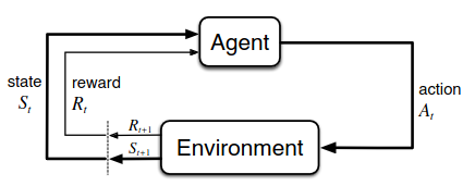
The agent and environment interact with each other in a sequence of discrete time steps $t = 0, 1, \dots, n.$ At each time step $t,$ the agent receives a representation of the environment's state $S_t \in \mathcal{S},$ and on that basis selects an action $A_t \in \mathcal{A}(s).$ At the next time step $t + 1,$ the agent receives a reward $R_{t + 1} \in \mathcal{R} \subset \mathbb{R}$ and finds itself in another state $s_{t+1}.$ Then, the MDP and agent give rise to a sequence or trajectory like this:

In a finite MDP, the random variables $R_t$ and $S_t$ have well defined discrete probability distributions that depend only on the previous state and action, i.e., for particular values of these random variables $s' \in \mathcal{A}, \ r \in \mathcal{R},$ there is a probability of those values occurring at time step $t,$ given particular values of the previous state and action:

The function $p: \mathcal{S} \times \mathcal{R} \times \mathcal{S} \times \mathcal{A} \rightarrow [0,1]$, which completely characterizes the MDP environment's dynamics, is an ordinary deterministic function with four arguments. This function $p$ specifies a probability distribution for each choice of $s$ and $a$, i.e.,

Markov property: the state must include information about all aspects of the past agent-environment interaction that make a difference for the future. In practice, this means that the probability of each possible value for $S_t$ and $R_t$ depends only on the previous state $S_{t-1}$ and action $A_{t-1}$.

• While most methods in this book assume this property to be true, there are methods that don't rely on it. Chapter 17 considers how to efficiently learn a Markov state from non-Markov observations.

From the dynamics function $p,$ we can compute the state-transition probabilities $p: \mathcal{S} \times \mathcal{S} \times \mathcal{A} \rightarrow [0,1],$

We can also compute the expected rewards for state-action pairs as a two-argument function $r : \mathcal{S} \times \mathcal{A} \rightarrow \mathbb{R}$:

and the expected rewards for the state-action-new_state triples as a three-argument function $r: \mathcal{S} \times \mathcal{A} \times \mathcal{S} \rightarrow \mathbb{R},$

Section 3.2: Goals and Rewards

In RL, the purpose of the agent is formalized in terms of a simple number, the reward (at each time step $R_t \in \mathbb{R}$), which passes from the environment to the agent. The agent's goal is to maximize the total cumulative reward, something stated in the reward hypothesis:

That all of what we mean by goals and purposes can be well thought of as the maximization of the expected value of the cumulative sum of a received scalar signal (called reward).

In order for the agent to achieve our goals, it is critical that the reward signals defined truly indicate what we want accomplished. Of particular importance, one must not use the reward signal to impart prior knowledge to the agent. Using chess as an example, we should naturally define the reward as $+1$ for winning, $-1$ for losing and $0$ for draws and all non-terminal positions. We should NOT give rewards for sub-goals like taking an opponent's chess piece, otherwise the agent might find a way to maximize its reward, even at the cost of losing the game. The reward signal defines what you want the agent to achieve, not how you want the agent to achieve it.

Section 3.3: Returns and Episodes

We seek to maximize the expected return, where the return $G_t$ is defined as some specific function of the reward sequence. In the simplest case the return is the sum of the rewards:

where $T$ is a final time step. This approach makes sense in applications where the agent-environment interaction can be naturally broken down into sub-sequences, called episodes, like the plays of a game or trips to a maze. Each episode ends in a special state, called the terminal state, and the resets to a starting state or a sample from standard distribution of starting states. Since the next episode begins independently of how the previous one ended, episodes can all be considered to end in the same terminal state, just with different rewards for different outcomes.

Episodic task: tasks that have discrete independent episodes, i.e., where the outcome of the ending of an episode doesn't effect the start state of the next episode.

• We sometimes distinguish the set of all non-terminal states $\mathcal{S}$ from the set of all states plus the terminal state $\mathcal{S}^+$;
• The time of termination $T$ is a random variable that can vary from episode to episode.

Continuing task: tasks where the agent-environment interaction cannot be naturally broken down into identifiable episodes, and goes on continually without limit.

• With the current formulation, the final time step for these tasks would be $T = \infty$ and thus, the total return we are trying to maximize could easily be infinite;
• To deal with this, we add the concept of discounting to the formulation. Now, the agent must try to select actions that maximize the sum of discounted rewards received.

Following this formulation, the agent must then chose $A_t$ s.t. the expected discounted return is maximal:

where $\gamma \in [0, 1]$ is a parameter called the discount rate. This parameter determines the current value of future rewards, i.e., a reward received $k$ time steps in future is only worth $\gamma^{k+1}$ times what it would be worth if it were received now. If $\gamma < 1$ and the reward sequence $\{R_k\}$ is bounded, then the infinite sum of discounted rewards has a finite value. If $\gamma = 0,$ the agent is only concerned with maximizing its immediate reward, i.e., its objective is to learn how to select $A_t$ s.t. it maximizes only $R_{t+1}.$ As $\gamma \rightarrow 1,$ the return objective takes future rewards more strongly into account, i.e., the agent becomes more farsighted. The returns at successive time steps are related to each other s.t.

This works for all time steps $t < T,$ even if the termination occurs at $t + 1,$ provided we define $G_T = 0$. If the reward is a constant $+1,$ then the return is

Section 3.4: Unified Notation for Episodic and Continuing Tasks

To be precise about episodic tasks, instead of considering one long sequence of time steps, we need to consider a series of episodes, where each episode consists of a finite sequence of time steps. As such, we refer to $S_{t, i}$ as the state representation at time step $t$ of episode $i$ (the same for $A_{t, i}, R_{t, i}, \pi_{t, i}, T_i, \dots$). In practice however, since we are almost always considering a particular episode or stating a fact that is true for all episodes, we can drop the explicit reference to the episode number.

We can unify the finite sum of terms for the total return in the episodic case and the infinite sum for the total reward in the continuing case by considering episode termination to be the entering of a special absorbing state that transitions only to itself and generates only rewards of zero, as exemplified in Figure 2.

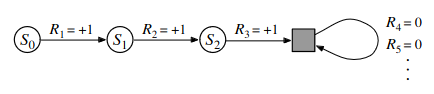
Including the possibility that $T = \infty \oplus \gamma = 1$ (where $\oplus$ is the XOR operator), we can write

Section 3.5: Policies and Value Functions

Value function: a function of states (or state-action pairs) that estimates how good it it is for the agent to be in a given state, defined in terms of future rewards that can be expected.

• Since the rewards the agent can expect to receive depend on what actions it takes, value functions are defined w.r.t. a particular way of acting, called a policy.

Policy: a mapping from states to probabilities of selecting each possible action, i.e., if the agent is following policy $\pi$ at time $t,$ then $\pi(a \vert s)$ is the probability that $A_t = a$ if $S_t = s.$

• It is a function that defines a probability distribution over $a \in \mathcal{A}(s)$ for each $s \in \mathcal{S}.$

The value function of a state $s$ under a policy $\pi,$ denoted $^{\pi}(s),$ is the expected return when starting in $s$ and following $\pi$ thereafter. For MDPs, $v^{\pi}$ can be formally defined as

where $\mathbb{E}_{\pi}[\cdot]$ denotes the expected value of random variable given that the agent follows policy $\pi,$ and $t$ is any time step (the value of the terminal state is always zero). The function $v^{\pi}$ is called the state-value function for policy $\pi$.

We can also define the value of taking action $a$ in state $s$ while following a policy $\pi,$ denoted $q^{\pi}(s, a),$ as the expected return starting from $s,$ taking the action $a,$ and following policy $\pi$ afterwards:

The function $q^{\pi}$ is called the action-value function for policy $\pi$. Both $q^{\pi}$ and $v^{\pi}$ can be estimated from experience, e.g., using Monte Carlo methods.

Monte Carlo methods: estimation methods that involve averaging over many random samples of a random variable.

• For examples, if an agent follows policy $\pi$ and maintains an average, for each state encountered, of the actual returns that have followed that state, then the average will converge to the state's actual value $v^{\pi}(s),$ as the number of times that state is encountered approaches infinity. If separate averages are kept for each action taken in each state, these averages will also converge to the action values $q^{\pi}(s, a)$;
• Since keeping an average for each state and state-action pair is usually not practical, the agent can instead maintain $v^{\pi}$ and $q^{\pi}$ as parameterized functions.

A fundamental property of commonly used value functions is that they satisfy recursive relationships similar to that of the return. For any policy $\pi$ and state $s,$ the following consistency condition holds between the value of $s$ and the value of its possible successor states:

where it is implicit that the actions $a$ are taken from the set $\mathcal{A},$ that the next state $s'$ are taken from the set $\mathcal{S}$ (or from $\mathcal{S}^+$ in the case of an episodic problem), and that the rewards $r$ are taken from the set $\mathcal{R}.$ The final expression, which is a sum over all values of the three variables $a$, $s'$, and $r$, can be read as an expected value. For each triple, we compute its probability $\pi(a \vert s) p(s', r \vert s, a),$ weight the quantity in brackets by that probability and then sum over all possibilities to get an expected value.

The last equation, called the Bellman equation for $v^{\pi}$, expresses a relationship between the value of a state and the values of its successor states (similar to a look-ahead). The Bellman equation averages over all the possibilities, weighting each by its probability of occurring, and it states that the value of the start state must equal the discounted value of the expected next state, plus the reward expected along the way. The value function $v^{\pi}$ is the unique solution to this equation.

Section 3.6: Optimal Policies and Optimal Value Functions

Solving a RL task roughly means finding a policy that maximizes the total reward over the long run. For finite MDPs, we can precisely define an optimal policy $\pi^*$ as follows:

• Value function define a partial ordering over policies;
• A policy $\pi$ is defined to be better than or equal to a policy $\pi'$, i.e., $\pi \geq \pi'$, iff $v^{\pi}(s) \geq v_{\pi'}(s), \ \forall s \in \mathcal{S}$;
• $\exists \pi^*: \pi^* \geq \pi, \ \forall \pi \in \mathcal{S}$.

Although there may be more than one optimal policy, we denote them all by $\pi^*$. They share the same state-value function, called the optimal state-value function, denoted $v^*$, and defined as

Optimal policies also share the same optimal action-value function, denoted $q^*$. For the state-action pair $(s, a)$, this function gives the expected return for taking action $a$ in state $s$ and following an optimal policy afterwards. This function can defined as

Section 3.7: Optimality and Approximation

Even if we have a complete and accurate model of the environment's dynamics, it is usually not possible to compute an optimal policy by solving the Bellman optimality equation. An important aspect of the problem is the amount of computational power available to the agent, in particular, the amount of computation it can perform in a single time step. Another important constraint is the memory available, specially since a large amount of memory is often required to build up approximations of value functions, policies, and models.

tabular case: task with small, finite state sets, which allow one to form approximations using arrays or tables with one entry for each state (or state-action pair), i.e., tabular methods.

• In tasks that have state sets too large to use tabular methods, we must instead rely on approximation using compact parameterized function representations.

The online nature of RL makes it possible to approximate optimal policies in ways that put more effort into learning to make good decisions for frequently encountered states, at the expense of less effort for infrequently encountered states.

Section 3.8: Summary

RL is about an agent learning how to behave in order to achieve a goal by interacting with its environment over a sequence of discrete time steps. The specification of their interface defines a particular task:

• Actions: choices made by the agent;
• States: the basis for making the choices;
• Rewards: the basis for evaluating the choices.

A policy is a stochastic rule by which the agent selects the actions as function of states. The optimal policy is that which best achieves the agent's objective, maximizing the amount of reward it receives over time.

The return is the function of future rewards that the agent seeks to maximize (in expected value). Its definition depends on the nature of the task and whether one wishes to discount delayed reward. The undiscounted formulation is appropriate for episodic tasks, and the discounted formulation is appropriate for tabular continuing tasks.

A policy's value functions ($v^*$ and $q^*$) assign to each state, or state–action pair, the largest expected return achievable by any policy. Whereas the optimal value functions are unique for a given MDP, there can be many optimal policies. In most cases, we seek approximations of the optimal value functions and policies, not their exact values.

Chapter 4: Dynamic Programming

The key idea of DP (and RL in general) is the use of value functions to both structure and organize the search for good policies. DP algorithms are obtained by turning Bellman equations into assignments, i.e., into update rules for improving approximations of the desired value functions. Remember that we can easily obtain optimal policies if we find the optimal value functions, $v^* \lor q^*$, which satisfy the Bellman optimality equations, $\forall s \in \mathcal{S}, \forall a \in \mathcal{A}(s), s' \in \mathcal{S}^+$, such that:

Section 4.1: Policy Evaluation (Prediction)

Policy evaluation: computing the state-value function $v^{\pi}$ for an arbitrary policy $\pi$. This is also referred to as the prediction problem. Recall from Chapter 3 that, $\forall s \in \mathcal{S}$,

where $\pi(a\vert s)$ is the probability of taking action $a$ in state $s$ under policy $\pi$, and the expectations are subscripted by $\pi$ to indicate that they are conditional on following policy $\pi$. If $\gamma < 1$ or eventual termination is guaranteed from all states under the policy $\pi$, then w.h.t. that $v^{\pi}$ exists and is unique.

def iterative_policy_evaluation(policy, mdp, theta, gamma):
    assert theta > 0;
    
    state_values[len(mdp.states)] = 0;
    for x in range(len(mdp.states) - 1):
        state_values[x] = random_value();
        
    gradient = 0;
    while gradient >= theta:
        gradient = 0;
        for s in mdp.states:
            v = state_values[s.id];
            state_values[s.id] = 0;
            for tmp_s in mdp.state:
                for a in mdp.actions:
                    state_values[s.id] += policy[s.id][a.id] * mdp.reward_probabilities(prev_state=s, cur_state=tmp_s, action=a) * (s.reward + gamma * state_values[state.id]);
            
            gradient = max(gradient, absolute_value(v - state_values[s.id]));

    return state_values;

Section 4.2: Policy Improvement

Knowing the value function $v^{\pi}$ for an arbitrary deterministic policy $\pi$, and given some state $s$, how can we determine whether or not we should change the policy to deterministically choose an action $a \neq \pi(s)$? One possible way, is to consider selecting $a$ in $s$ and afterwards following the existing policy $\pi$. The value of this manner of behaving is given by:

The key criterion is whether this is greater than or less than $v^{\pi}$. If it is greater, i.e., if it is better to select $a$ once in $s$ and thereafter follow $\pi$ than it is to always follow $\pi$, then one can expect that it would be better to select $a$ ever time $s$ is encountered, and that such new policy would be a better one overall. This fact is a special case of a general result called the policy improvement theorem.

Let $\pi$ and $\pi'$ be any pair of deterministic policies s.t.:

Then the policy $\pi'$ must be as good as, or better than, $\pi$, i.e., it must obtain greater or equal expected return from all states:

Additionally, if there is strict inequality of $q^{\pi}(s, \pi'(s))$ at any state, then there must be strict inequality of $v^{\pi'}(s)$ at that state. This theorem applies to the two policies considered: a deterministic policy $\pi$, and a changed policy $\pi'$, identical to $\pi$ in everything except $\pi'(s) = a \neq \pi(s)$. Since $v^{\pi'} = v^{\pi}, \forall s' \in \mathcal{S} \setminus \{s\},$ if $q^{\pi}(s, a) > v^{\pi}(s)$, then the changed policy $\pi'$ must be better than $\pi$.

In order to understand the idea of the proof behind the policy improvement theorem, we can start from $q^{\pi}(s, \pi'(s)) \geq v^{\pi}(s)$, then keep expanding the l.h.s. with the equation for $q^{\pi}(s, a)$ and reapplying $q^{\pi}(s, \pi'(s)) \geq v^{\pi}(s)$:

Now knowing how, given a policy policy and its value function, to evaluate a change in the policy at a single, we to extend this result to consider changes at all states - selecting at each state the action that appears best according to $q^{\pi}(s, a)$, i.e., to consider the new greedy policy $\pi'$, given by

The greedy policy takes the action that looks best according to $v^{\pi}$ after a single step of lookahead. Since, by construction, the greedy policy meets the conditions of the policy improvement theorem, we know that it is as good as - or better than - the original policy.

Policy improvement: process of making a new policy that improves on an original policy by making it greedy w.r.t. the value function of the original policy.

Supposing that the new greedy policy $\pi'$ is as good as, but not better than, the old policy $\pi$, then $v^{\pi}(s) = v^{\pi'}$, and, $\forall s \in \mathcal{S}$, it follows from the previous equation that

As this is the same as the Bellman optimality equation, $v^{\pi'}$ must be $v^*$, and both $\pi$ and $\pi'$ must be optimal policies. Thus, policy improvement must give us a strictly better policy except when the original policy is already optimal.

The policy improvement theorem carries through as stated for the stochastic case. Also, if there are any ties in policy improvement steps - i.e., there are several actions at which the maximum is achieved - then we don't need to select a single action from among them, as each maximizing action can be given a portion of the probability of being selected in the new greedy policy (as long as we give zero probability to all submaximal actions).

Section 4.3: Policy Iteration

A policy $\pi$ can be iteratively improved to yield a better policy, thus leading to a sequence of monotonically improving policies and value functions:

where $\xrightarrow{E}$ denotes a policy evaluation and $\xrightarrow{I}$ a policy improvement. Each policy is guaranteed to be a strict improvement over the previous one, unless it is already an optimal policy. Since a finite MDP has a finite number of deterministic policies, this process must converge to an optimal policy and the optimal value function in a finite number of iterations.

This way of finding an optimal policy is called policy iteration. Each policy evaluation is started with the value function for the previous policy, which usually results in a great increase in the algorithm's speed of converge (presumably due to the fact that the value function changes little from one policy to the next).

def policy_evaluation(policy, mdp, state_values, theta, gamma):
    gradient;
    while gradient >= theta:
        gradient = 0;
        for s in mdp.states:
            value = state_values[s.id];
            state_values[s.id] = 0;
            for tmp_s in mdp.states:
                state_values[s.id] += mdp.reward_probabilities(prev_state=s, cur_state=tmp_s, action=argmax(policy[tmp_s.id])) * (mdp.reward + gamma * state_values[tmp_s.id]);
                
            gradient = max(gradient, absolute_value(value - state_values[s.id]))

    return state_values;

    def policy_improvement(policy, mdp, gamma):
        policy_stable = True;
        
        for s in mdp.states:
            old_action = argmax(policy[s.id]);
            for tmp_s in mdp.states:
                policy[s.id] = mdp.reward_probabilities(prev_state=s, cur_state=tmp_s, action=) * (mdp.reward + gamma * state_values[tmp_s.id]);
            
            if old_action != argmax(policy[s]):
                policy_stable = False;

        return policy, policy_stable;

    def policy_iteration(mdp, theta, gamma):
        assert theta > 0;
        
        state_values[len(mdp.states)];
        state_values[len(mdp.states)] = 0;
        policy[len(mdp.states)][len(mdp.actions)];
        for x in range(len(mdp.states) - 1):
            state_values[x] = random_value();
            for y in range(len(mdp.actions)):
                policy[x][y] = random_value();

            // Since a policy is probabilities, its values must sum to 1
            policy[x] = (policy[x] - min(policy[x]) / (max(policy[x]) - min(policy[x]))


        policy_stable = False;
        while (!policy_stable):
            state_values = policy_evaluation(policy, mdp, state_values, theta, gamma)
            policy, policy_stable = policy_improvement(policy, mdp, gamma)

    return policy

Section 4.4: Value Iteration

A drawback of policy iteration is that it may involve several policy evaluations, which can be a protracted computation in itself. If policy evaluation is done iteratively, then convergence to exactly $v^{\pi}$ occurs only at the limit. However, we can often truncate policy evaluation, e.g., policy evaluation iterations beyond the first three have no effect on the corresponding greedy policy.

The policy evaluation step of policy iteration can be truncated in several ways without losing the algorithm's convergence guarantees. One special case is when policy evaluation is stopped after just one sweep (one update of each state). This algorithm, which is called value iteration, can be written as a simple update operation that combines the policy improvement and truncated policy evaluation steps:

For an arbitrary $v_0$, the sequence $\{v_k\}$ can be shown to converge to $v*$ under the same conditions that guarantee the existence of $v^*$. Note that value iteration is obtained simply by turning the Bellman optimality equation into an update rule. Also, note how the value iteration update is identical to the policy evaluation update, except that it requires the maximum to be taken over all actions.

def value_iteration(mdp, theta, gamma):
    assert theta > 0;

    state_values[len(mdp.states)];
    state_values[len(mdp.states)] = 0;
    policy[len(mdp.states)];
    for x in range(len(mdp.states) - 1):
        state_values[x] = random_value();
        policy[x] = 0;

    gradient;
    while gradient >= theta:
        gradient = 0;
        for s in mdp.states:
            old_value = state_values[s.id];
            tmp_value[len(mdp.states)];
            for tmp_s in mdp.state:
                for a in mdp.actions:
                    tmp_value[tmp_s.id] += mdp.reward_probabilities(prev_state=s, cur_state=tmp_s, action=a) * (state.reward + gamma * state_values[state.id]);

            state_values[s.id] = max(tmp_value);
            gradient = max(gradient, absolute_value(old_value - state_values[s.id]));

    for s in mdp.states:
        tmp_value[len(mdp.states)];
        for tmp_s in mdp.state:
            for a in mdp.actions:
                tmp_value[tmp_s.id] += mdp.reward_probabilities(prev_state=s, cur_state=tmp_s, action=a) * (state.reward + gamma * state_values[state.id]);

        policy[s.id] = argmax(tmp_value);

    return policy;

In each of its sweeps, value iteration combines one sweep of policy evaluation and one of policy improvement. Faster convergence is often achieved by interposing multiple policy evaluation sweeps between each policy improvement sweep. Since the max operation is the only difference between these updates, this just means that the max operation is added to some sweeps of policy evaluation. All of these algorithms converge to an optimal policy for discounted finite MDPs.

Section 4.5: Asynchronous Dynamic Programming

A significant drawback to the previously discussed DP methods is the fact that they involve operations over the entire state set of the MDP, i.e., they require sweeps of the state set. As such, a single sweep can become prohibitively expensive, e.g., in the game of backgammon (that has $10^{20}$ states), even if we could perform the value iteration update on a million states per second, it would still take $1000+$ years to complete a single sweep.

Asynchronous DP algorithm: in-place iterative DP algorithm that is not organized in terms of systematic sweeps of the state set, i.e., the values of some states may be updated several times before the values of others are updated even once.

• To convergence correctly, such an algorithm must continue to update the values of all the state, i.e., it can't ignore any state after some point in the computation;
• Doesn't need to get locked into any hopelessly long sweep before making progress improving a policy, allowing one to order the updates s.t. value information efficiently propagates from state to state (some ideas for this are introduced in Chapter 8);
• Can be run at the same time that an agent is actually experience the MDP, meaning that the agent's experience can be used to determine which states to update and the value and policy information can guide the agent's decision making.
  • Ex: apply updates to states as the agents visits them, thus focusing the algorithm's updates onto the parts state set parts most relevant to the agent.

Example (sweepless DP) algorithm: update the value, in place, of only one state $s_k$ on each step $k$, using the value iteration update.

• If $0 \leq \gamma < 1$, asymptotic convergence to $v^*$ is guaranteed given only that all states occur in the sequence $\{s_k\}$ an infinite number of times;
• It is possible to intermix policy evaluation and value iteration updates to produce a kind of asynchronous truncated policy iteration.

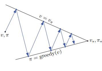
Section 4.6: Generalized Policy Iteration

Policy iteration consists of two simultaneous and interacting processes:

• Policy evaluation: makes the value function consistent with the current policy;
• Policy improvement: makes the policy greedy w.r.t. the current value function.

These two processes need not be alternate and/or completed one after the other, since, as long as both processes continue to update all states, convergence to the optimal value function and (an) optimal policy is guaranteed.

Generalized policy iteration (GPI): the general idea of letting policy evaluation and policy improvement processes interact, independent of the details of the two processes. Almost all RL methods can be described as GPI, i.e., they have identifiable policies and value functions, with the policy always being improved w.r.t. the value function, and the value function always being driven toward the value function for the policy.

If both the evaluation process and the improvement process stabilize, then the value function and policy must be optimal. The value function only stabilizes when it is consistent with the current policy, and the policy stabilizes only when it is greedy with respect to the current value function. This implies that the Bellman optimality equation, which means that the policy and the value function are guaranteed to be optimal.

Section 4.7: Efficiency of Dynamic Programming

While DP methods may not be the most practical solution for very large problems they can be quite efficient when compared with other methods for solving MDPs. If $n$ and $k$ denote the number of states and actions, respectively, a DP method takes less computational operations than some polynomial function of $n$ and $k$ to find an optimal policy, even though the total number of (deterministic) policies is $k^n$.

Direct search and linear programming methods can also be used to solve MDPs, and in some cases their worst-case convergence guarantees are even better than those of DP methods. However, linear programming methods become impractical at a much smaller number of states than DP methods do (by a factor of about 100).

While DP methods may seem of limited applicability due to the curse of dimensionality (the fact that the number of states often grows exponentially with the number of state variables), in practice, such methods can be used with today's computers to solve MDPs with millions of states. Also, these methods normally converge much faster than their theoretical worst-case runtimes, specially if they are started with good initial value functions or policies. For very large state spaces, asynchronous DP are often preferred.

Section 4.8: Summary

Policy evaluation refers to the (usually) iterative computation of the value functions for a given policy. In turn, policy improvement refers to the computation of an improved policy given the value function for that policy. Putting these two together forms the backbone of the two most popular DP methods, policy iteration and value iteration.

Classical DP methods involve sweeps of expected update operations over each state of the state set. They are little more than the Bellman operations turned into assignment statements. Convergence occurs once the updates no longer result in changes in value.

Almost all RL methods can be viewed as a form of GPI: one process takes the policy as given and performs some form of policy evaluation, changing the value function to be more like the true value function for the policy; and the other process takes the value function as given (assuming its the policy's value function) and performs some form of policy improvement, changing the policy to make it better.

Asynchronous DP methods are iterative methods that updates states in an arbitrary order, possibly stochastic and using out-of-date information.

Bootstrapping: general idea of updating estimates based on other estimates.

• DP methods perform this as they update the estimates of the values of states based on the estimates of the values of successor states;
• Many RL methods also perform this, even those that - unlike DP methods - do not require a complete and accurate model of the environment.

Chapter 5: Monte Carlo Methods

Monte Carlo (MC) method: an estimation method that obtain results by computing the average of repeated random samples. For RL, this means computing the average of complete returns (as opposed to methods that learn from partial returns).

• Requires only experience, i.e., sample sequences of states, actions, and rewards from an actual or simulated interaction with an environment;
• Value estimates and policy changes are only computed when an episode terminates;
• To ensure that well-defined returns are available, here we define MC methods only for episodic tasks (i.e., experience is divided into episodes that eventually terminate).

Learning from actual experience is a very powerful tool, since it requires no prior knowledge of the environment's dynamics, yet can still achieve optimal behavior. Learning from simulated experience is also powerful, although a model is required to generate sample transitions (unlike in DP, which requires a complete probability distribution of all possible transitions).

MC methods sample and average returns for each state-action pair, similarly to the bandit methods of Chapter 2. The main difference is that there are now multiple different bandit problems which are all interrelated, i.e., the return after taking an action is one state depends on the actions taken in later states of the same episode (making the problem non-stationary from the P.o.V. of the earlier state). We adapt the idea of GPI to handle the non-stationarity, where instead of computing value function from knowledge of the MDP, we learn value functions from sample return with the MDP.

Section 5.1: Monte Carlo Prediction

Recall that the value of a state is the expected return - expected cumulative future discounted reward - starting from that state. The idea of estimating the expected return by averaging the returns observed after visits to that state underlies all MC methods. Each occurrence of a state $s$ in an episode is called a visit to $s$, and the first time it is visited in an episode is called the first visit to $s$.

The first-visit MC method estimates $v^{\pi}(s)$ as the average of the returns following first visits to $s$, whereas the every-visit MC method averages the returns following all visits to $s$. By the law of large numbers, both methods converge to $v^{\pi}(s)$ as the number of (first-)visits to $s$ goes to infinity. The two methods are similar, but have slightly different theoretical properties. Every-visit MC extends more naturally to function approximation and eligibility traces.

def first_visit_monte_carlo_prediction(policy, gamma, mdp):
    returns[len(mdp.states)] = [];
    state_values[len(mdp.states)];
    state_values[len(mdp.states)] = 0;
    for x in range(len(mdp.states) - 1):
        state_values[x] = random_value();

    while(True):
        episode = generate_episode_following_policy(policy, mdp);
        G = 0;
        for step in episode[:0:-1]:
            G = gamma * G + step.reward;
            if step.state not in episode[:-1]:
                returns[step.state.id].append(G);
                state_value[step.state.id] = mean(returns)

Section 5.2: Monte Carlo Estimation of Action Values

Without a model, one must explicitly estimate the value of each action in order for the values to be useful in suggesting a policy. As such, one the primary goals for MC methods is to estimate $q^*$. The policy evaluation problem for action values is to estimate $q^{\pi}(s, a)$, i.e., the expected return when starting in state $s$, taking action $a$, and thereafter following policy $\pi$.

A state-action pair $(s, a)$ is said to be visited in an episode if ever the state $s$ is visited and action $a$ is taken in it. The every-visit MC method estimates the value of a state–action pair as the average of the returns that have followed all the visits to it. In turn, the first-visit MC method averages the returns following the first time in each episode that the state was visited and the action was selected.

If $\pi$ is a deterministic policy, then in following it one will observe returns only for one of the actions from each state, and with no returns to average, the MC estimates of the other actions will not improve with experience. This is a serious problem, since to alternatives we need to estimate the value of all the actions from each state, not just the one we currently favor.

This is the general problem of maintaining exploration, as discussed in Chapter 2. For policy evaluation to work for action values, we must assure continual exploration. One way to do this is by assuming exploring starts, which means that the episodes start in a state–action pair, and that every pair has a nonzero probability of being selected as the start.

The previous assumption cannot always be relied upon, particularly when learning directly from actual interaction with an environment. The most common alternative approach to assuring that all state–action pairs are encountered is to consider only policies that are stochastic with a nonzero probability of selecting all actions in each state.

Section 5.3: Monte Carlo Control

Chapter 6: Temporal-Difference Learning

Chapter 7: $n$-step Bootstrapping

Chapter 8: Planning and Learning with Tabular Methods

Part II: Approximate Solution Methods

Chapter 9: On-policy Prediction with Approximation

Chapter 10: On-policy Control with Approximation

Chapter 11: *Off-policy Methods with Approximation

Chapter 12: Eligibility Traces

Chapter 13: Policy Gradient Methods

Notation relevant for this chapter:

• Policy's parameter vector: $\theta \in \mathbb{R}^{d'}$;
• Learned value function's weight vector: $w \in \mathbb{R}^d$;
• Scalar performance measure w.r.t. the policy parameter: $J(\theta)$;
• Probability that action $a$ is taken at time $t$, given that the environment is in state $s$ at time $t$: $\pi (a \vert s, \theta) = P (A_t = a|S_t = s,\theta_t = \theta)$.

Policy gradient methods seek to learn an approximation to the policy by maximizing performance. Their updates approximate gradient ascent such as:

Methods that learn an approximation of both policy and value functions are called actor-critic methods. The actor is a reference to the learned policy and critic a reference to the learned (state-)value function.

Section 13.1: Policy Approximation and its Advantages

The policy can be parameterized in any way, as long as 2 conditions are met

• As long as $\pi(a\vert s, \theta)$ is differentiable w.r.t. its parameters:

• As long as it continues to perform exploration (to avoid a deterministic policy):

For small-to-medium discrete action spaces, it is common to form parameterized numerical preferences $h(s, a, \theta) \in \mathbb{R}$ for each $(s, a)$ pair. The probabilities of each action being selected can be calculated with, e.g., an exponential softmax distribution:

This kind of policy parameterization is called softmax in action preferences.

The action preferences can be parameterized arbitrarily, e.g., as the output of a Deep Neural Network (DNN) with parameters $\theta$. They can also be linear in features:

The choice of policy parameterization can be a good way of injecting prior knowledge about the desired form of the policy into the RL system. Beyond this, parameterizing policies according to the softmax in action preferences has several advantages:

• Allows the approximate policy to approach a deterministic policy, unlike with $\epsilon$-greedy action selection (due to the $\epsilon$ probability of selecting a random action);
• Enables the selection of actions with arbitrary probabilities (useful if the optimal policy is a stochastic policy, e.g., in a game of chance such as poker);
• If the policy is easier to approximate then the action-value function, then policy-based methods learn faster and yield a superior asymptotic policy.

Section 13.2: The Policy Gradient Theorem

Policy parameterization has an important theoretical advantage over $\epsilon$-greedy action selection: the continuity of the policy dependence on the parameters that enables policy gradient methods to approximate gradient ascent.

Due to the continuous policy parameterization the action probabilities change smoothly as a function of the learned parameters, unlike with $\epsilon$-greedy selection, where the action probabilities may change dramatically if an update changes which action has the maximal value.

In the episodic case, the performance measure is defined as the value of the start state of the episode. Taking a (non-random) state $s_0$ as the start state of the episode and $v_{\pi_{\theta}}$ as the true value function for the policy $\pi_{\theta}$, the performance can be defined as:

Since the policy parameters affect both the action selections and the distribution of states in which those selections are made, and performance also depends on both, it may be challenging to to change the policy parameters such that improvement is ensured, particularly since the effect of the policy on the state distribution is a function of the environment, and thus is typically unknown.

The policy gradient theorem provides a solution towards this challenge in the manner of an analytic expression for the gradient of performance w.r.t. the policy parameters, without the need for the derivative of the state distribution. The equation for episodic case of the policy gradient theorem is given by:

where $\mu$ is the on-policy distribution under $\pi$. For the episodic case, the constant of proportionality is the average length of an episode, and for the continuing case it is 1.

Section 13.3: REINFORCE: Monte Carlo Policy Gradient

Since any constant of proportionality can be absorbed into the step size $\alpha$, all that is required is a way of sampling that approximates the policy gradient theorem. As the r.h.s. of the theorem is a sum over states weighted by their probability of occurring under the target policy $\pi$, w.h.t.:

Thus, we can instantiate the stochastic gradient ascent algorithm (known as the all-actions method, due to its update involving all of the actions) as:

where $\hat{q}$ is a learned approximation of $q^{\pi}$. Unlike the previous method, the update step at time $t$ of the REINFORCE algorithm involves only $A_t$ (the action taken at time $t$). By multiplying and then dividing the summed terms by $\pi (a\vert S_t, \theta)$, we can introduce the weighting needed for an expectation under $\pi$., then, given that $G_t$ is the return, w.h.t.:

Since the final (in brackets) expression is a quantity that can be sampled on each time step with expectation proportional to the gradient, such a sample can be used to instantiate the generic stochastic gradient ascent algorithm, yielding the REINFORCE update:

where $\gamma$ is the discount factor and $\ln \pi(A_t|S_t, \theta_t)$ is the eligibility vector. In this update, each increment is proportional to the return - causing the parameters to move most in the directions of the actions that yield the highest return - and is inversely proportional to the action probability - since the most frequent selected actions would have an advantage otherwise.

Since REINFORCE uses the complete return from time $t$ (including all future rewards until the end of an episode), it is considered a Monte Carlo algorithm and is only well defined in the episodic case with all updates made in retrospect after the episode's completion.

As a stochastic gradient method, REINFORCE assures an improvement in the expected performance (given a small enough $\alpha$) and convergence to a local optimum (under standard stochastic approximation conditions for decreasing $\alpha$). However, as a Monte Carlo method, REINFORCE may have high variance and subsequently produce slow learning.

def episodic_reinforce(policy, environment, alpha, gamma):
    assert alpha > 0;
    policy.theta = initialize_policy_parameters();
    while(True):
        episode = environment.generate_episode();
        for step in episode:
            G = sum([R_k * gamma**(k-step.t-1) for k, R_k in enumerate(episode.rewards]));
            policy.theta += alpha * gamma**step.t * G * compute_gradient(log(policy[step.state][step.action]));

Section 13.4: REINFORCE with Baseline

Generalizing the policy gradient theorem to include a comparison of the action value to an arbitrary baseline $b(s)$ gives the following expression:

The baseline can be any arbitrary function (as long as it doesn't vary with $a$), since the equation will remain valid as the subtracted quantity is zero:

The theorem can then be used to derive an update rule similar to the previous version of REINFORCE, but which includes a general baseline:

While the baseline generally leaves the expected value of the update unchanged, it can have a significant effect on its variance and thus the learning speed.

The value of the baseline should follow that of the actions, i.e., if all actions have high/low values, then the baseline must also have high/low value, so as to differentiate the higher valued actions from the lower valued ones. A common choice for the baseline is an estimate of state value $\hat{v}(S_t, w)$, with $w \in \mathbb{R}^d$ being a learned weight vector.

The algorithm has two step sizes, $\alpha_{\theta}$ (which is the same as the step size $\alpha$ in previous equations) and $\alpha_{w}$. A good rule of thumb for setting the step size for values in the linear case is

The step size for the policy parameters $\alpha_{\theta}$ will depend on the range of variation of the rewards and on the policy parameterization.

def episodic_reinforce_wbaseline(policy, state_value_function, environment, alpha_theta, alpha_w, gamma):
    assert alpha_theta > 0;
    assert alpha_w > 0;
    policy.theta = initialize_policy_parameters();
    state_value_function.w = initialize_state_value_parameters();
    while(True):
        episode = environment.generate_episode();
        for step in episode:
            G = sum([R_k * gamma**(k-step.t-1) for k, R_k in enumerate(episode.rewards]));
            delta = G - state_value_function(step.state);
            state_value_function.w += alpha_w * delta * compute_gradient(state_value_function(step.state));
            policy.theta += alpha_theta * gamma**step.t * delta * compute_gradient(log(policy[step.state][step.action]);)

Section 13.5: Actor-Critic Methods

In actor-critic methods, the state-value function is applied to the second state of the transition, unlike in REINFORCE, where the learned state-value function only estimates the value of the first state of each state transition and thus can´t be used to assess that action. After discount and adding the estimated value of the second state to the reward, it constitutes the 1-step return $G_{t:t+1}$, which can be used to assess the action.

Even though the 1-step return introduces bias, it is often superior to the actual return in terms of its variance and computational congeniality. The bias can also be flexibly modulated through $n$-step returns and eligibility traces.

1-step actor-critic methods are analogs of the TD methods such as TD(0), Sarsa(0) and Q-learning. Such methods are appealing since they function in fully online and incremental manner, while avoiding the complexities of eligibility traces. In these methods, the full return of REINFORCE is replaced with the 1-step return (with a state-value function as the baseline) as follows:

A usual state value function learning method to pair with this is semi-gradient TD(0). To generalize to the forward view of $n$-steps methods and to a $\lambda$-return, one only needs to replace the on-step return in the previous equation by $G_{t:t+1}$ or $G_t^{\lambda}$, respectively. The backward view of the $\lambda$-return algorithm is also simple, only requiring using separate eligibility traces for the actor and critic.

def episodic_one_step_actor_critic(policy, state_value_function, environment, alpha_theta, alpha_w, gamma):
    assert alpha_theta > 0;
    assert alpha_w > 0;
    policy.theta = initialize_policy_parameters();
    state_value_function.w = initialize_state_value_parameters();
    while(True):
        s = environment.initialize();
        I = 1;
        while s.not_terminal():
            a = policy[s];
            next_state = environment.get_next_state(s, a);
            if next_state.is_terminal():
                value = 0;
            else:
                value = state_value_function[next_state];
            delta = environment.get_reward(s, a) + gamma * value;
            state_value_function.w += alpha_w * delta * compute_gradient(state_value_function[step.state]);
            policy.theta += alpha_theta * I * delta * compute_gradient(log(policy[step.state][step.action]));
            I = gamma * I;
            s = next_state;

    def episodic_actor_critic_with_traces(policy, state_value_function, environment, lambda_theta, lambda_w, alpha_theta, alpha_w, gamma):
        assert 1 >= lambda_theta >= 0;
        assert 1 >= lambda_w >+ 0;
        assert alpha_theta > 0;
        assert alpha_w > 0;
        policy.theta = initialize_policy_parameters();
        state_value_function.w = initialize_state_value_parameters();
        while(True):
            s = environment.initialize();
            z_theta = 0;
            z_w = 0;
            I = 1;
            while s.not_terminal():
                a = policy[s];
                next_state = environment.get_next_state(s, a);
                if next_state.is_terminal():
                    value = 0;
                else:
                    value = state_value_function[next_state];
                delta = environment.get_reward(s, a) + gamma * value - state_value_function[s];
                z_w = gamma * lambda_w * z_w + compute_gradient(state_value_function[step.state]);
                z_theta = gamma * lambda_theta * z_theta + I * compute_gradient(log(policy[step.state][step.action]));
                state_value_function.w += alpha_w * delta * z_w;
                policy.theta += alpha_theta * delta * z_theta;
                I = gamma * I;
                s = next_state;

Section 13.6: Policy Gradient for Continuing Problems

For continuing problems without episode boundaries, the performance must be defined in terms of the average rate of reward per time step:

where $\mu$ is the steady-state distribution under $\pi$, $\mu(s) \doteq \lim_{t \rightarrow \infty} P(S_t = s \vert A_{0:t} \sim \pi)$, which is assumed to exist and - due to the ergodicity assumption - to be independent of $S_0.$ This is a special distribution under where, if you select actions according to $\pi$, you remain in the same distribution, as follows:

In the continuing case, we define values: $v^{\pi} (s) \doteq \mathbb{E}_{\pi} (G_t \vert S_t = s)$ and $q^{\pi}(s, a) \doteq \mathbb{E} [G_t \vert S_t = s, A_t = a]$, w.r.t. the differential return (s.t. the policy gradient theorem holds true for the continuing case):

def continuing_actor_critic_with_traces(policy, state_value_function, environment, lambda_theta, lambda_w, alpha_theta, alpha_w, alpha_R):
    assert 1 >= lambda_theta >= 0;
    assert 1 >= lambda_w >+ 0;
    assert 1 >= lambda_R >+ 0;
    assert alpha_theta > 0;
    assert alpha_w > 0;
    R_bar = random_value();
    policy.theta = initialize_policy_parameters();
    state_value_function.w = initialize_state_value_parameters();
    s = environment.initialize();
    z_theta = 0;
    z_w = 0;
    while(True):
        a = policy[s];
        next_state = environment.get_next_state(s, a);
        delta = environment.get_reward(s, a) - R_bar + state_value_function[next_state] - state_value_function[s];
        R_bar += alpha_R * delta;
        z_w = lambda_w * z_w + compute_gradient(state_value_function[s]);
        z_theta = lambda_theta * z_theta + compute_gradient(log(policy[step.state][step.action]));
        state_value_function.w += alpha_w * delta * z_w;
        policy.theta += alpha_theta * delta * z_theta;
        s = next_state;

Section 13.7: Policy Parameterization for Continuous Actions

In policy-based methods, instead of computing learned probabilities for each and every action, instead we learn statistics of the probability distribution, e.g., the action set might be $\mathbb{R}$, with actions chosen from a normal (Gaussian) distribution. The Probability Density Function (PDF) for this (normal) distribution can be written as

where $\mu$ is the mean and $\sigma$ the standard deviation of the normal distribution, and $\pi \approx 3.14159$.

In order to make a policy parameterization, the policy may be defined as the normal probability density over a real-valued scalar action, with $\mu$ and $\sigma$ given by the parametric function approximators that depend on the state, i.e.,

where $\mu: \mathcal{S} \times \mathbb{R}^{d'} \rightarrow \mathbb{R}$ and $\sigma : \mathcal{S} \times \mathbb{R}^{d'} \rightarrow \mathbb{R}^+$ are two parameterized function approximators. Now, we just need to give a form for these approximators. To do this, we divide the policy's parameters into two parts, i.e., $\theta = [\theta_{\mu}, \theta_{\sigma}]$, one part will be used to approximate $\mu$ and the other to approximate $\sigma > 0$, the latter of which is better approximated as the exponential of a linear function. Thus

where $x_{\mu}(s)$ and $x_{\sigma}(s)$ are state feature vectors. With these additional definitions, all previously described algorithms can be applied to learn to select real-valued actions.

Section 13.8: Summary

Prior to this chapter: focus on action-value methods - which are methods that learn action values and then use them to select actions.

During this chapter: describes methods that learn parameterized policies that enable actions to be taken without consulting action-value estimates, with a focus on policy-gradient methods - which are methods that, on each step, update the policy parameter in the direction of an estimate of the gradient of the performance w.r.t. the policy parameter.

Advantages of methods that learn and store a policy parameter:

• They can learn specific probabilities for taking actions;
• They can learn appropriate levels of exploration and approach deterministic policies asymptotically;
• They can inherently handle continuous action spaces;
• The policy may be simpler to represent parametrically than the value function on some problems;
• The policy gradient theorem provides an exact formula (that doesn't involve derivatives of the state distribution) for how performance is affected by the policy parameter.

A state-value function baseline reduces the variance of the REINFORCE method without introducing bias. If the state-value function is (also) used to assess the policy's action selections, then it is called a critic, the policy is called an actor, and the overall algorithm is called an actor-critic method. The critic introduces bias into the actor’s gradient estimates, but this is often desirable since it substantially reduces variance (similar to the advantage bootstrapping TD methods have over Monte Carlo methods).

Part III: Looking Deeper

Chapter 14: Psychology

Chapter 15: Neuroscience

Chapter 16: Applications and Case Studies

Chapter 17: Frontiers